Excel Tips & Tricks: Effortlessly Highlight Entire Rows with Conditional Formatting Techniques

Quick Links

• Step One: Create Your Table
• Step Two: Format Your Table
• Step Three: Create The Conditional Formatting Rules

Conditional formatting lets you format cells in an Excel spreadsheet based on the cells’ content. For example, you could have a cell turn red when it contains a number lower than 100. You can also use conditional formatting to highlight an entire row?

Related: Using Conditional Cell Formatting in Excel 2007

If you’ve never used Conditional Formatting before, you might want to look at Using Conditional Cell Formatting in Excel 2007 . It’s for an earlier version of Excel, but the interface really hasn’t changed much. That guide talks about formatting specific cells based on their content. For example, say you use a spreadsheet to track hours that employees have worked. You could use conditional formatting to color cells red where an employee has worked more than eight hours in a particular day.

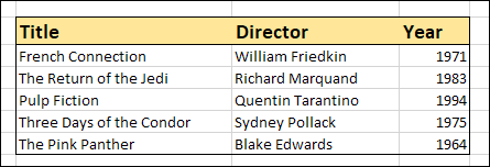
But what if you wanted to use a cell’s value to highlight other cells? In the example we’re using for this article, we’ve got a small spreadsheet with movies and just a couple of details about those movies (to keep thinks simple). We’re going to use conditional formatting to highlight all the rows with movies made before 1980.

Step One: Create Your Table

Obviously, the first thing you need is a simple table containing your data. The data doesn’t have to be text-only; you can use formulas freely. At this point, your table has no formatting at all:

Step Two: Format Your Table

Now it’s time to format your table, if you want. You can use Excel’s “simple” formatting tools or take a more hands-on approach, but it’s best only to format only those parts that won’t be affected by conditional formatting. In our case, we can safely set a border for the table, as well as format the header line.

Step Three: Create The Conditional Formatting Rules

Now we come to the meat and potatoes. As we said at the outset, if you’ve never used conditional formatting before, you should probably check out our earlier primer on the subject and once you’ve got that down, come back here. If you’re already somewhat familiar with conditional formatting (or just adventurous), let’s forge on.

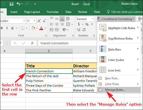
Select the first cell in the first row you’d like to format, click the “Conditional Formatting” button in the “Styles” section of the “Home” tab, and then select “Manage Rules” from the dropdown menu.

Epubor Ultimate for Mac:Helps you read books anywhere, including the best eBook Converter + eBook DRM Removal functions.

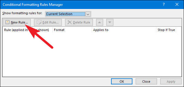
In the “Conditional Formatting Rules Manager” window, click the “New Rule” button.

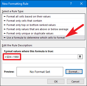
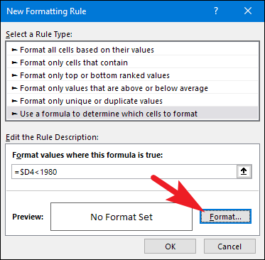
In the “New Formatting Rule” window, select the “Use a formula to determine which cells to format” option. This is the trickiest part. Your formula must evaluate to “True” for the rule to apply, and must be flexible enough so you could use it across your entire table later on. Here, we’re using the formula:

=$D4<1980

The =$D4 part of the formula denotes the address of the cell I want to examine. D is the column (with the movie release date), and 4 is my current row. Note the dollar sign before the D . If you don’t include this symbol, then when you apply conditional formatting to the next cell, it would examine E5. Instead, you need to specify have a “fixed” column ($D) but a “flexible” row (4), because you are going to apply this formula across multiple rows.

The <1980 part of the formula is the condition that has to be met. In this case, we’re going for a simple condition—the number in the release date column should be less than 1980. Of course, you can use much more complex formulas if you need to.

So in English, our formula is true whenever the cell in column D in the current row has a value less than 1980.

Next, you’ll define the formatting that happens if the formula is true. In the same “New Formatting Rule” window, click the “Format” button.

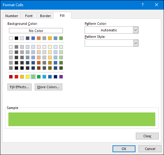
In the “Format Cells” window, go through the tabs and tweak the settings until you get the look you want. In our example, we’re just going to change the fill color to green on the “Fill” tab. When you’re done applying your formatting, click the “OK” button.

OtsAV DJ Pro

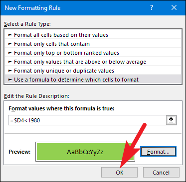
Back in the “New Formatting Rule” window, you can now see a preview of your cell. If you’re happy with the way everything looks, click the “OK” button.

You should now be back to the “Conditional Formatting Rules Manager” window. Move the window a bit until you can see your spreadsheet behind it, and then click the “Apply” button. If the formatting of your selected cell changes, that means your formula is correct. If the formatting doesn’t change, you need to go a few steps back and tweak your formula until it does work. Here, you can see that our formula worked, and the cell we selected is now filled in green.

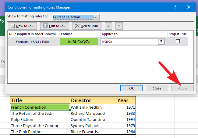
Now that you have a working formula, it’s time to apply it across the entire table. As you can see above, right now the formatting applies only to the cell we started off with. In the “Conditional Formatting Rules Manager” window (which should still be open), click the up arrow to the right of the “Applies To” field.

The “Conditional Formatting Rules Manager” window collapses, giving you access to your spreadsheet. Drag to resize the current selection across the entire table (except for the headings).

When you’re done, click the down arrow to the right of the address field to get back to the full “Conditional Formatting Rules Manager” window.

Note that the “Applies to” field now contains a range of cells instead of just a single address. Click the “Apply” button again, and you should see the whole table formatted according to your rule. In our example, you can see that the whole rows that contain movies made before 1980 are filled with green.

That’s it! If you have more complex needs, you can create additional formulas. And, of course, you can make your formulas a whole lot more complex than the simple example we’ve used here. You can even use conditional formatting between different spreadsheets, so that cells or rows in one spreadsheet are formatted differently depending on the data in a whole different sheet. Play around with the techniques we’ve covered, and in no time you’ll be creating intricate spreadsheets with data that pops right off the screen.