
Mastering Microsoft Excel: A Comprehensive Guide on Leveraging the Subtotal Formula

Mastering Microsoft Excel: A Comprehensive Guide on Leveraging the Subtotal Formula
Quick Links
Key Takeaways
To use the SUBTOTAL function, create a formula using the syntax: SUBTOTAL(function_number, reference 1, reference 2,…). You can also use the Subtotal feature by selecting your rows, then clicking the “Data” tab. In the Outline drop-down menu, select “Subtotal.”
Obtaining subtotals for groups of related items is easy in Microsoft Excel. In fact, you have two ways to do this. You can either use the SUBTOTAL function or the Subtotal feature, whichever works best. We’ll show you how.
What Is a Subtotal in Excel?
As mentioned, SUBTOTAL in Excel allows you to group the same or related items in a list and use a function to calculate the values. For example, you can use it to sum sales by month or average grades by student. You could also add inventory by product or count the number of bills due next week.
Using the SUBTOTAL function by creating a formula or using the Subtotal feature, you can get the calculations you need in just a few steps.
Use the Excel SUBTOTAL Function
You can create a formula using the Excel SUBTOTAL function with the flexibility to include or exclude rows you’ve hidden.
The syntax for the formula is
`SUBTOTAL(function_number, reference 1, reference 2,...)`
where the first two arguments are required. You can use additional cell references or named ranges for the remaining arguments as needed.
The
`function_number`
argument allows you to insert one of 11 functions using its corresponding number. The first 11 include hidden rows, while the second 11 exclude them. So, simply insert the number for the function you need and how you want to handle the hidden rows.
| Function | Include Hidden Rows | Exclude Hidden Rows |
|---|---|---|
| AVERAGE | 1 | 101 |
| COUNT | 2 | 102 |
| COUNTA | 3 | 103 |
| MAX | 4 | 104 |
| MIN | 5 | 105 |
| PRODUCT | 6 | 106 |
| STDEV | 7 | 107 |
| STDEVP | 8 | 108 |
| SUM | 9 | 109 |
| VAR | 10 | 110 |
| VARP | 11 | 111 |
As an example of the SUBTOTAL function, we’ll sum the total of sales in the cell range B2 through B4 using this formula:
=SUBTOTAL(9,B2:B4)
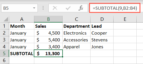
For this next example, we hid rows 4 and 5. Using this first formula, we can obtain our sum using the number 9 for the first argument to include the hidden data.
=SUBTOTAL(9,B2:B6)
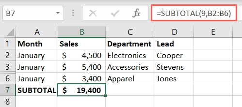
Now, we’ll exclude those hidden rows from our total, using the number 109 for our first argument.
=SUBTOTAL(109,B2:B6)
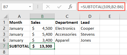
Once you have your subtotals, you can use the SUBTOTAL function once more for a grand total at the bottom. Alternatively, you can use the SUM function to add the subtotals.
Related: How to Sum a Column in Microsoft Excel
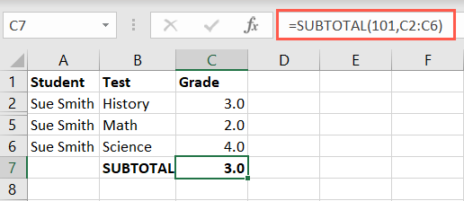
For another example, we’ll use the average function to include hidden rows 3 and 4 with this formula:
=SUBTOTAL(1,C2:C6)
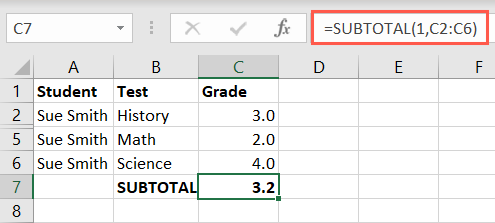
And next, we’ll exclude the hidden rows with this formula:
=SUBTOTAL(101,C2:C6)
Notes on the SUBTOTAL Function
Here are a few things to keep in mind when using the SUBTOTAL function in Excel:
- The function works for columns or vertical ranges, not rows or horizontal ranges.
- If you have nested subtotals in the reference argument area, Excel ignores these in the subtotal result.
- When you use a filter , the data filtered out is excluded from the subtotal result.
Use the Subtotal Feature
Another way to use the SUBTOTAL function in Excel is by using the Subtotal feature. This way, you can automatically add calculations and group the items at the same time. Excel uses the SUBTOTAL function to accomplish this for you. Let’s look at a couple of examples.
Related: How to Calculate Workdays With a Function in Microsoft Excel
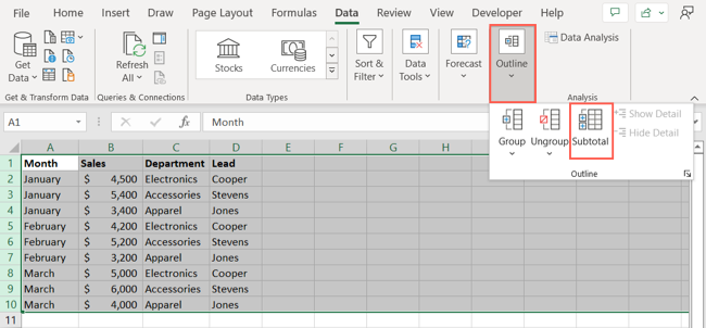
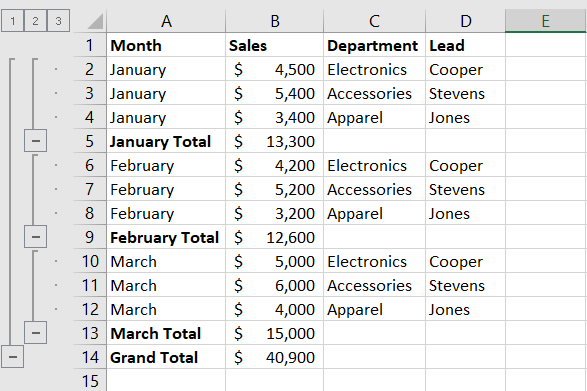
Using the Subtotal feature for our sales by month, we can group the data per month and sum each group with a grand total at the bottom.
Select all of the rows you want to group and subtotal. Go to the Data tab and pick “Subtotal” in the Outline drop-down menu.
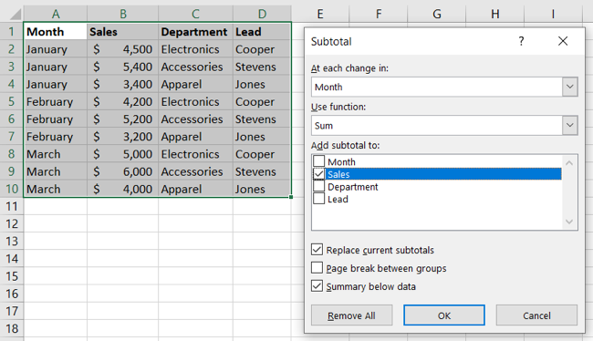
When the Subtotal box opens, choose how you want to add the subtotals.
- At Each Change In : Select the column you want to use for the grouping. Here, we picked Month so that a new group is created when the Month changes in the sheet.
- Use Function : Select the function you want to use, such as sum, average, minimum, maximum, or another option. For our example, we selected Sum.
- Add Subtotal to : Check the box for where you want the subtotal to calculate. For our example, we picked Sales.
Optionally check the boxes at the bottom for the additional items as you like. Click “OK.”
You’ll then see your data update to group and subtotal the rows and create a grand total at the bottom. Use the plus, minus, and number buttons to collapse or expand the groups for easier viewing.
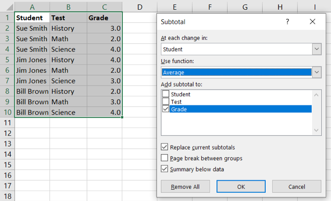
As another example, we’ll use student grades. We’ll use the Subtotal and Group features to display an average grade for each student. Here’s the process.
Select the rows, go to Data, and pick “Subtotal” in the Outline drop-down menu.
In the Subtotal box, we’ll choose Student in the change drop-down list and Average in the function list. We’ll then check the box for Grade. Click “OK.”
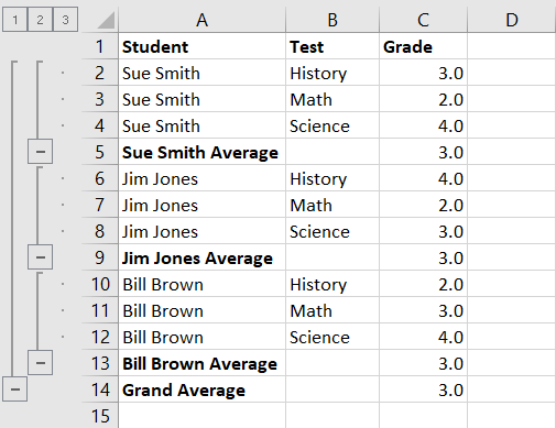
We now have our rows grouped by student with an average grade for each and an overall average at the bottom. Again, you can use the buttons on the left to collapse and expand the groups.
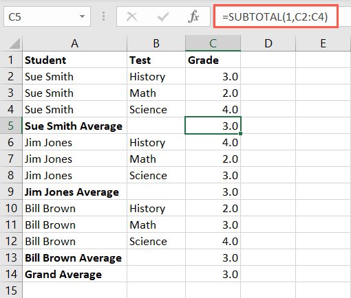
If you decide to ungroup the rows after you use the Subtotal feature, the rows return to normal. However, those containing the SUBTOTAL function used by Excel remain for you to continue using or simply delete if you prefer.
The Subtotal feature can become complex if you plan to use many groups. However, these basic examples should help get you started if you’re interested in this function.
One thing to note is that you can’t add an Excel table subtotal with this feature. If you have your data in a table, you can either insert the Excel formula for SUBTOTAL as described earlier or convert your table to a cell range to use the feature. If you choose the latter, you’ll lose the table functionality.
Now that you know how to insert subtotals in Excel, check out how to remove duplicate rows .
| | Mastering Excel Functions | | |
| —————————- | ——————————————————————————————————————————————————————————————————————————————————————————————————————————————————————————————————————————————————————————————————————————————————————————————————————————————————————————————————————————————————————————————————————————————————————————————————————————————————————————————————————————————————————————————————————————————————————————————————————————————————————————————————————————————————————————————————————————————————————————————————————————————————————————————————————————————————————————————————————————————————————————————————————————————————————————————————————————————————————————————————————————————————————————————————————————————————————————————————————————————————————————————————————————————————————————————————————————————————————————————————————————————————————————————————————————————————————————————————————————————————————————————————————————————————————————————————————————————————————————————————————————————————————————————————————- | |
| Functions | AVERAGE · CONCATENATE · COUNT · COUNTIF · DATEDIF · FILTER · FREQUENCY · FV · HYPERLINK · IF · IFS · IMAGE · INDEX · IS · LEN · MATCH · MEDIAN · RAND · ROUND · RRI · SORT · SQRT · SUBSTITUTE · SUBTOTAL · SUM · SUMIF · TODAY · TRIM · TRUNC · VLOOKUP · WEEKDAY · XLOOKUP · YEAR | |
| Types | Basic · Budgeting · Data Entry · Logical · Text · Time and Date | |
| Explained | Copying Formulas · Evaluating Formulas · Finding Functions · Fixing Formula Errors · Functions vs Formulas · Comparing Lookup Functions · Locking Formulas · Structuring Formulas · Translating Formulas | |
Also read:
- [New] 2024 Approved Download Free MCB Logo Templates
- [New] Wildlife Wonders at Fingertips Top Mobile Simulators for 2024
- [Updated] Is Paying Monthly for YouTube's Unlimited Access a Good Deal, In 2024
- 2024 Approved Subscriber Threshold Raised for Profits
- End Minecraft Game Freezing - Discover 6 Quick Solutions to Stabilize Your Playtime
- Enhance Your Printing with the Newest DYMO LabelWriter E-4XL Driver
- Fix Your PC: Troubleshooting Steps When Fuser Continuously Crashes
- From Queens to the Big Screen: The Impact of Miles Morales in Marvel's Latest Game
- In 2024, How to Get and Use Pokemon Go Promo Codes On Samsung Galaxy XCover 7 | Dr.fone
- Mastering Splitgate Graphics Settings: Fixes for Increasing Speed & Reducing Stutter
- Solve Endless Loading on Anthem: A Comprehensive Fix Guide
- Ultimate Guide to Increasing Your ARK: Sanctuary's Performance - Tips for PC Players
- Understanding and Fixing the Persistent ntdll.dll System Crashes in Modern Operating Systems
- Video File Repair - How to Fix Corrupted video files of Vivo V29 Pro?
- Title: Mastering Microsoft Excel: A Comprehensive Guide on Leveraging the Subtotal Formula
- Author: Paul
- Created at : 2024-12-04 17:08:36
- Updated at : 2024-12-06 16:36:33
- Link: https://win-able.techidaily.com/mastering-microsoft-excel-a-comprehensive-guide-on-leveraging-the-subtotal-formula/
- License: This work is licensed under CC BY-NC-SA 4.0.