
Unlock Excel Efficiency: A Comprehensive Tutorial on Freezing/Thawing Rows & Columns

Unlock Excel Efficiency: A Comprehensive Tutorial on Freezing/Thawing Rows & Columns
Quick Links
- Freeze the Top Row
- Freeze the Left Row
- Freeze Your Own Group of Rows or Columns
- Freeze Columns and Rows at the Same Time
If you are working on a large spreadsheet, it can be useful to “freeze” certain rows or columns so that they stay on screen while you scroll through the rest of the sheet.
As you’re scrolling through large sheets in Excel, you might want to keep some rows or columns—like headers, for example—in view. Excel lets you freeze things in one of three ways:
- You can freeze the top row.
- You can freeze the leftmost column.
- You can freeze a pane that contains multiple rows or multiple columns—or even freeze a group of columns and a group of rows at the same time.
So, let’s take a look at how to perform these actions.
Freeze the Top Row
Here’s the first spreadsheet we’ll be messing with. It’s the Inventory List template that comes with Excel, in case you want to play along.
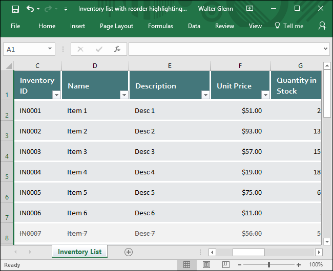
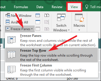
The top row in our example sheet is a header that might be nice to keep in view as you scroll down. Switch to the “View” tab, click the “Freeze Panes” dropdown menu, and then click “Freeze Top Row.”
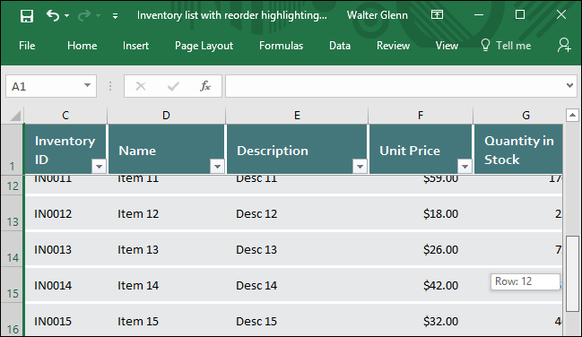
Now, when you scroll down the sheet, that top row stays in view.
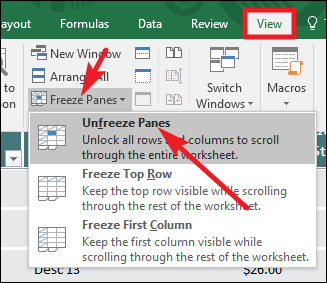
To reverse that, you just have to unfreeze the panes. On the “View” tab, hit the “Freeze Panes” dropdown again, and this time select “Unfreeze Panes.”
Freeze the Left Row
Sometimes, the leftmost column contains the information you’ll want to keep on screen as you scroll to the right on your sheet. To do that, switch to the “View” tab, click the “Freeze Panes” dropdown menu, and then click “Freeze First Column.”
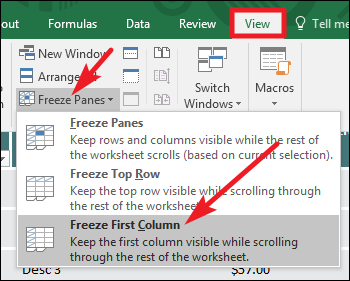
Now, as you scroll to the right, that first column stays on screen. In our example, it lets us keep the inventory ID column visible while we scroll through the other columns of data.
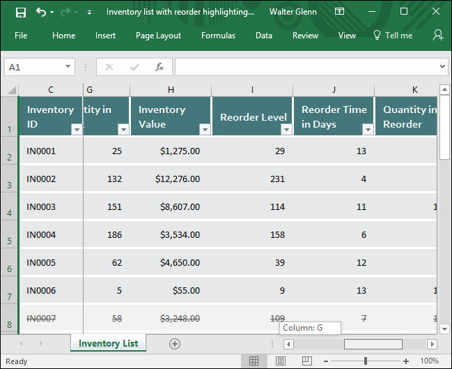
And again, to unfreeze the column, just head to View > Freeze Panes > Unfreeze Panes.
Freeze Your Own Group of Rows or Columns
Sometimes, the information you need to freeze on screen isn’t in the top row or first column. In this case, you’ll need to freeze a group of rows or columns. As an example, take a look at the spreadsheet below. This one is the Employee Attendance template included with Excel, if you want to load it up.
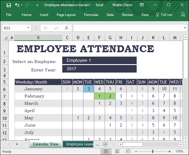
Notice that there are a bunch of rows at the top before the actual header we might want to freeze—the row with the days of the week listed. Obviously, freezing just the top row won’t work this time, so we’ll need to freeze a group of rows at the top.
First, select the entire row below the bottom most row that you want to stay on screen. In our example, we want row five to stay on screen, so we’re selecting row six. To select the row, just click the number to the left of the row.
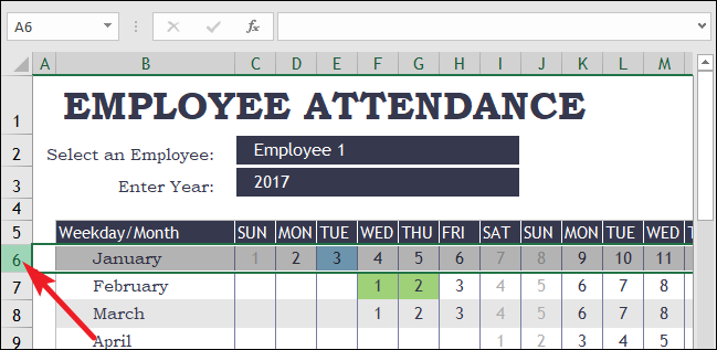
Next, switch to the “View” tab, click the “Freeze Panes” dropdown menu, and then click “Freeze Panes.”
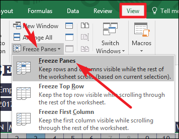
Now, as you scroll down the sheet, rows one through five are frozen. Note that a thick gray line will always show you where the freeze point is.

To freeze a pane of columns instead, just select the whole row to the right of the right most row you want to freeze. Here, we’re selecting Row C because we want Row B to stay on screen.

And then head to View > Freeze Panes > Freeze Panes. Now, our column showing the months stays on screen as we scroll right.

And remember, when you have frozen rows or columns and need to return to a normal view, just go to View > Freeze Panes > Unfreeze Panes.
Freeze Columns and Rows at the Same Time
We have one more trick to show you. You’ve seen how to freeze a group of rows or a group of columns. You can also freeze rows and columns at the same time. Looking at Employee Attendance spreadsheet again, let’s say we wanted to keep both the header with the weekdays (row five) and the column with the months (column B) on screen at the same time.
To do this, select the uppermost and leftmost cell that you don’t want to freeze. Here, we want to freeze row five and column B, so we’ll select cell C6 by clicking it.

Next, switch to the “View” tab, click the “Freeze Panes” dropdown menu, and then click “Freeze Panes.”

And now, we can scroll down or right while keeping those header rows and columns on screen.

Freezing rows or columns in Excel isn’t difficult, once you know the option is there. And it can really help when navigating large, complicated spreadsheets.
Also read:
- [Updated] Designing a Simple YouTube Subscriber Shortcut
- Beat Helldivers 2 on Computer: Expert Fixes for Uninterrupted Gaming Bliss
- Beating Diablo II Resurrected Stability Problems – Fixes Unveiled
- Demystifying Google Hangouts: Origin, Features, and Evolution Over Time
- Edit and Send Fake Location on Telegram For your Xiaomi Redmi K70 Pro in 3 Ways | Dr.fone
- Elevate Your The Ascent Adventure: Proven Strategies to Reduce Stuttering & Increase FPS Performance
- Fixing Gameplay Interruptions: Tips for Smoother Rocket League Experience
- In 2024, A Comprehensive Walkthrough of Adobe Presenter Recording
- In 2024, How to Screen Mirroring Oppo Reno 11 5G to PC? | Dr.fone
- In 2024, Ways To Find Unlocking Codes For Oppo Reno 8T Phones
- Navigating YouTube's Creative Commons Framework Effectively for 2024
- Solving the Issue: Reducing God of War's Excessive CPU Demand
- Troubleshooting Guide: Fixing 'Battle.net Launcher' Issues on Windows PCs
- What Makes Periscope Special? Understanding Features & Registration
- Where Is the Best Place to Catch Dratini On Realme Narzo 60 5G | Dr.fone
- Title: Unlock Excel Efficiency: A Comprehensive Tutorial on Freezing/Thawing Rows & Columns
- Author: Paul
- Created at : 2024-12-10 16:08:55
- Updated at : 2024-12-12 16:43:27
- Link: https://win-able.techidaily.com/unlock-excel-efficiency-a-comprehensive-tutorial-on-freezingthawing-rows-and-columns/
- License: This work is licensed under CC BY-NC-SA 4.0.