Unlocking Excel's Secrets: 11 Uncommon Yet Essential Features for Enhanced Efficiency

Unlocking Excel’s Secrets: 11 Uncommon Yet Essential Features for Enhanced Efficiency

Quick Links

Microsoft Excel offers hundreds of functions . So, there’s bound to be at least a handful you don’t know exist. These unique functions have specific purposes that you’ll be thrilled to learn about and use.

FLOOR and CEILING for Rounding

You can use the FLOOR and CEILING math functions for rounding towards or away from zero by a specified multiple. Use FLOOR to round down and CEILING to round up.

The syntax for each is

    `FLOOR(value, multiple)`

and

    `CEILING(value, multiple)`

where both arguments are required.

To round 4.4 down to the nearest multiple of 2, you’d use the following formula:

=FLOOR(4.4,2)

To round 5.6 up to the nearest multiple of 2, you’d use this formula:

=CEILING(5.6,2)

MODE.SNGL for Finding Repetitive Values

Originally simply the MODE function , Microsoft created a newer version of this statistical function for improved accuracy. Use MODE.SNGL to find a single frequently recurring number in an array or cell range.

The syntax is MODE.SNGL(array1, array2, ...) where only the first argument is required. You can use numbers, names, arrays, or references that contain numbers. Use the optional argument(s) for additional cell ranges.

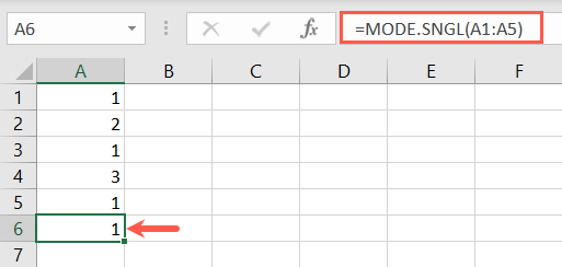
Here, we look for the repetitive number that appears the most in cells A1 through A5.

=MODE.SNGL(A1:A5)

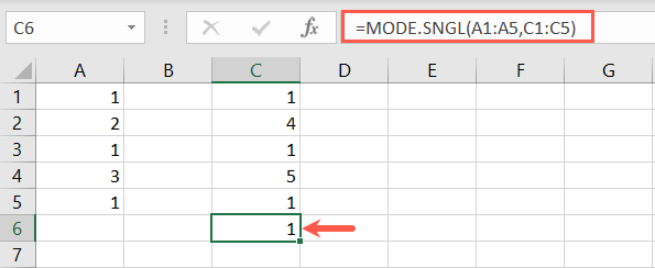
To find a recurring number in A1 through A5 and C1 through C5, you’d use this formula:

=MODE.SNGL(A1:A5, C1:C5)

CONVERT for Converting From One Measurement to Another

For a useful engineering function, you can use CONVERT to change a value from one measurement system to another.

The syntax is CONVERT(value, from, to) where you’ll need all three arguments. For the from and to arguments, you’ll use an abbreviation. Check the Microsoft Support site for the abbreviations you need for weight and mass, distance, time, pressure, force, energy, power, magnetism, temperature, volume, area, information, and speed.

To convert the value in cell A1 from Celsius to Fahrenheit, you would use this formula:

=CONVERT(A1,”C”,”F”)

vMix Pro - Software based live production. vMix Pro includes everything in vMix 4K plus 8 channels of Replay and 8 vMix Call
This bundle includes Studio 200 for vMix from Virtualsetworks, HTTP Matrix 1.0 automation scheduler, and 4 introductory training videos from the Udemy vMix Basic to Amazing course.

To convert the value in cell B1 from centimeters to inches, use this formula:

=CONVERT(B1,”cm”,”in”)

DELTA for Testing Equal or Not Equal Values

Another engineering function that’s useful is DELTA. With it, you’ll use the Kronecker delta function to test whether two values are equal. Different than the EXACT function , the result is either 1 (true) or 0 (false).

The syntax is DELTA(value1, value2) where only the first argument is required and can be a number or cell reference. If you leave the second argument blank, Excel assumes zero.

To test the values in cells A1 and B1, you would enter this formula:

=DELTA(A1,B1)

To test the values 2 and -2, use this formula:

=DELTA(2,-2)

GESTEP for Testing Greater Than or Equal To a Threshold

One more engineering function you may find useful is GESTEP which allows you to test values that are greater than or equal to a step (threshold). The result is either 1 (true) or 0 (false).

The syntax is GESTEP(value, step) where only the first argument is required and can be a number or cell reference. If you leave the second argument blank, Excel uses zero.

To test the value in cell A1 against step 4, you’d use this formula:

=GESTEP(A1,4)

To test a value of 10 against step 12, use this formula:

=GESTEP(10,12)

ADDRESS for Finding the Location of a Cell

Let’s move on to a lookup function in Excel. To find the exact address of a cell, you can use the ADDRESS function. This is convenient if you want an error-free reference to a cell .

The syntax is ADDRESS(row, column, type, style, name) where only the first two arguments are required. Enter the row number for the first argument and the column number for the second.

The optional arguments are as follows:

Type: The type of reference to return. Use blank or 1 for absolute, 2 for absolute row and relative column, 3 for relative row and absolute column, or 4 for relative.
Style: Use TRUE for the A1 or FALSE for the R1C1 cell reference style .
Name: The sheet name to use for an external reference. If blank, Excel assumes the currently active sheet.

To find the address of the cell in row 2, column 3, you’d use this formula:

=ADDRESS(2,3)

To find the address of the same cell using an absolute row and relative column, you’d use this formula:

=ADDRESS(2,3,2)

To find the address of the same cell in the sheet named Sheet2, use the following formula. Note that the commas represent the blank arguments type and style.

=ADDRESS(2,3,,,”Sheet2”)

Click here

## PI for the Value of Pi

If you need to use the value of pi for equations in your sheet, you can obtain it with the PI function.

The syntax is simply PI() with no arguments. You can add more elements to the formula if you want to use the value for a calculation.

To return the value of pi, simply use the function’s formula including the parentheses:

=PI()

To multiply the value of pi by 10, you’d use this formula:

=PI()*10

ARABIC and ROMAN for Converting Numerals

Another math function you may find handy is for converting to and from Arabic and Roman numerals .

The syntax for each is ARABIC(text) and ROMAN(value, form) where the first argument is required for each.

The optional argument for the ROMAN function specifies the type of Roman numeral from Classic to Simplified. Enter the number 0, word TRUE, or omit the argument for Classic. Use a 1, 2, or 3 for a more concise result. Or, enter the number 4 or the word FALSE for Simplified.

To convert the Roman numeral MMIM to an Arabic number, use this formula making sure to include the text in quotes:

=ARABIC(“MMIM”)

To convert 2,999 to a Roman numeral, you’d use this formula:

=ROMAN(2999)

To convert the same number in Simplified form, use one of these formulas:

=ROMAN(2999,4)

=ROMAN(2999,FALSE)

REPT for Entering Repeating Text

If you want to add a series of characters, symbols, or text as a placeholder or for a visual effect, use the REPT text function .

The syntax is REPT(text, number) where both arguments are required. Enter the text argument within quotes and then the number of times to repeat that text.

To repeat the word Excel 10 times in a cell, you’d use this formula:

=REPT(“Excel”,10)

Epubor Audible Converter for Mac： Download and convert Audible AAXC/AA/AAX to MP3 with 100% original quality preserved.

To repeat an asterisk 20 times, you’d use this formula:

=REPT(“*”,20)

vMix Basic HD - Software based live production. vMix Basic HD includes 4 inputs, 3 cameras, streaming, recording, playlist.
This bundle includes Studio 200 for vMix from Virtualsetworks, HTTP Matrix 1.0 automation scheduler, and 4 introductory training videos from the Udemy vMix Basic to Amazing course.

We’ve covered many Excel functions at How-To Geek and try to walk you through using the most common options. Hopefully one of these out-of-the-ordinary functions is exactly what you need for math, engineering, statistical, lookup, or textual data.

| | Mastering Excel Functions | | |
| —————————- | —————————————————————————————————————————————————————————————————————————————————————————————————————————————————————————————————————————————————————————————————————————————————————————————————————————————————————————————————————————————————————————————————————————————————————————————————————————————————————————————————————————————————————————————————————————————————————————————————————————————————————————————————————————————————————————————————————————————————————————————————————————————————————————————————————————————————————————————————————————————————————————————————————————————————————————————————————————————————————————————————————————————————————————————————————————————————————————————————————————————————————————————————————————————————————————————————————————————————————————————————————————————————————————————————————————————————————————————————————————————————————————————————————————————————————————————————————————————————————————————————————————————————————————————————————— | |
| Functions | AVERAGE · CONCATENATE · COUNT · COUNTIF · DATEDIF · FILTER · FREQUENCY · FV · HYPERLINK · IF · IFS · IMAGE · INDEX · IS · LEN · MATCH ·MEDIAN · RAND · ROUND · RRI · SORT · SQRT · SUBSTITUTE · SUBTOTAL · SUM · SUMIF · TODAY · TRIM · TRUNC · VLOOKUP · WEEKDAY · XLOOKUP · YEAR | |
| Types | Basic · Budgeting · Data Entry · Logical · Text · Time and Date | |
| Explained | Copying Formulas · Evaluating Formulas · Finding Functions · Fixing Formula Errors · Functions vs Formulas · Comparing Lookup Functions · Locking Formulas · Structuring Formulas · Translating Formulas | |

Win Able